Linux for terrified biologists

Genome analysis survival guide

Preface - What is this?

This document started as my notes for the Genome analysis course taught by Dr. Flegontov, that I took at the University of Ostrava in 2016. Soon I turned it into a short tutorial for my classmates (and my supervisor, then interested in learning the subject). I still update it every now and then, so it’s work in progress. You can comment on stuff you would like to clarify or expand and I’ll try my best to improve it.

I’m by NO means an expert. On the contrary - I’m far from the level of dr. Flegontov, only maybe a few lessons ahead of other students in the group.

But precisely for this reason I know the struggles of beginners, because they are still in my memory (some quite alive). I went through similar problems recently and I think it might have helped if I had something akin to this small tutorial at hand. Google can be overwhelming at times, right? :)

Update: Originally I started with Google Docs, this version uses Markdown and Github Pages instead.

Connection

For setting up connection to linux server you need Eduroam or similar open network (your home wifi is fine too), because osu-simple allows only http(s) protocol (i.e. web). You can get all the necessary info on the university website.

There you will also find a link to special tools that will set the network for you (works on Windows, Linux, Mac and even Android and iOS).

password: needs to be set on Portal (it’s special for eduroam only).

SSH - secure shell

To connect from Windows you need ssh client, e.g. the simple Putty or the advanced MobaXterm. There you will fill the login details.

To connect from Linux you just open Terminal (try pressing Ctrl+Alt+T) and type command in this form:

ssh -p 22 studentuser@genome.osu.cz

The number after -p is port; 22 is default and can be omitted, but you can be told to use different port.

To connect from Mac you also just open Terminal and type something like this:

ssh studentuser@genome.osu.cz -p22

To disconnect from ssh session you can either type exit, press Ctrl+d, or simply close the window of your client.

First linux commands

Looking around

So you have successfully connected to some linux machine (server) and now you want to look around. You see a bunch of text on a black screen, now what? If you look down at the bottom line, it says something like:

studentuser@ubuntu2:~$

This is the infamous linux command line and it waits for your input (that is the $ symbol at the end - if you see it there, you can type your commands next to it).

To look around, type:

ls # lists contents of current folder

which will show content of a folder you are in. If you are familiar with R statistical environment you might notice it looks like R command ls(). And indeed it has similar function. You might also notice the # with comment after it - that’s also similar to R. I will use it to comment on what something does - if you copy it into the command line with the command, nothing extra happens, just as in R ;) Everything between # and new line (Enter) is ignored by linux.

Now you can do some stuff with what you see in the folder, like:

cp # copy
mv # move (cut+paste; can be used as rename)
rm # remove (delete)
mkdir # make directory (folder)
cd # change directory (go through folders)
pwd # path to working (current) directory (i.e. where you are)

So if you want to go into subdirectory, you can just type e.g. cd Jena and you will get there. If you want to go back (up), you just type

cd .. # two dots mean directory above in hierarchy

You can enter the path to the folder in several ways, some more lazy than others:

cd Jena # change to subfolder of current folder, named 'Jena'
cd ./Jena/ # same as above, using full relative path syntax
cd /home/studentuser/Jena # same as above, using absolute path
cd / # change to root directory of the system (like C:/)
cd ~ # go home ;) i.e. /home/studentuser

💡️ Tip: one dot represents directory you are currently in. That’s sometimes used for running scripts etc.

To copy file into some subdirectory, just type:

cp file.txt Jena/ # copies file.txt into Jena directory
cp file.txt Jena/renamed.txt # rename file during transfer

💡️ Tip: If you want to recall previous command, press arrow up (like in R). Now you can modify it and confirm with Enter. Also, if you start typing name of file/folder like Je.. and hit Tab, it will fill in the rest of the name - magic! :) But only if there is nothing else starting with the same letters Je.. - in such case hit Tab second time and it will tell you what other files match what you type. That’s double magic, my friend :)

ls Jena # check content of subfolder without going there

Command parameters

Now you can also add some parameters to commands, e.g.:

ls -l # lists content of current folder with details like size

Helpful manuals

Every command tool has its manual, which lists all the parameters and other useful info about the command. It’s very similar to R help. In R you type ?ls or help(ls) while in linux you can get it like this:

man ls # shows manual page of the command ls

This is probably the most helpful thing you will find here :)

💡️ Tip: the manual opens in interactive mode so you can move the page with arrows etc. Press Q to quit the manual page ;)

Syntax

You may have noticed a few similarities with the R language. Linux command line actually uses its own language called bash (but can easily use some others, like awk or perl).

In R you have syntax like this:

function(parameter1=value1, par2=value2, ...) # R syntax

The same in bash would be:

function --parameter value # bash syntax

Many parameters have shortcuts which look like this:

function -p value # shorter version

💡️ Tip: You can find both long and short version in the man page of particular command.

Let’s try something more. In R you can see objects in the environment with ls() but you can also save its result into new object like this:

x <- ls() # R version of creating dummy object

Basically what you do is that you redirect output of a function from standard output (stdout, typically your screen) into an object. The logic of bash is very similar:

ls > x # bash version creates file x with content from ls

I’m showing the preferred syntax, but you can actually switch sides in R:

ls() -> x # this is valid R operation

So the analogy between the two languages becomes more obvious.

💡️ Tip: note that linux bash syntax is case sensitive (just like R) so file.txt and File.txt are two different files.

Hello world

And speaking of syntax, what about the famous “Hello world!” program? This is usually the first program you learn in a new language, as it’s one of the simplest possible. It should just print Hello world! on the screen. In bash, this is as simple as:

echo Hello world! # the Hello world program

Notice that unlike most scripting languages, the command used is not print.

Playing with files and stuff

Standard output and redirecting

There are some useful day-to-day commands that work with text-based files (ASCII, i.e. you can reasonably open them in notepad and read them, e.g. txt or fasta files). These commands print output to stdout (screen) but you can save the output into file (as above) or redirect it into another command with pipes (in a moment):

wc # word count
wc -l # counts lines (rows) instead of words
head # shows first few rows of a file
tail # shows last few rows of the file
head -10 # shows first 10 rows
cat # concatenate (join) two or more files by rows
paste # the same but by columns (not so straightforward though)
grep 'pattern' # filter lines (rows) containing “pattern”

If you use cat with just one file, it will just print it on your screen, which is useful in many workflows. You can for example do this:

cat alignment.fasta | wc -l > file.txt # counts number of lines in alignment.fasta and saves result into file.txt

This is the famous unix | pipe. It takes standard output (stdout) of one command (here cat) and uses it as standard input (stdin) of another command (here wc).

💡️ Tip: one > symbol will create new file or overwrite existing one. If you want to append output to the end of existing file instead of overwriting it, you can use >>.

You can already do something useful with these, for example count number of sequences inside your fasta file (each sequence starts with “>” as you probably know):

cat alignment.fasta | grep '>' | wc -l # gives number of sequences in alignment.fasta file

💡️ Tip: stdin and stdout are example of classic programming terminology and it may be handy to know such stuff when you google for solution to your problems. In many scenarios stdout is your screen and stdin is your keyboard (if you don’t redirect them). There is also standard error (stderr), which is sometimes used as second output, typically to print error messages (but can be used for other purposes too).

Quoting and escaping

There are many special symbols and reserved words in bash, used all the time in commands and scripts. But sometimes you need to remove the special meaning. This is done by quoting or escaping.

In some cases you can’t really do without quotes (or the solution is way more complicated than just using quotes), in some other cases they are rather recommended good practice, that can save you from disasters in edge cases. Escaping is mostly used when you want to disable special meaning for a single character. This is done by prepending the target character with backslash \.

But let’s get real. Consider this simple example of printing sequence names from fasta file:

grep > alignment.fasta # BAD BAD VERY BAD!!!
grep '>' alignment.fasta # OKAY

Now grep doesn’t require quotes around pattern to work. But it’s a good practice to use them, as this example shows. The problem here is with the special character >. The first command interprets it as redirection and basically saves empty input in your alignment.fasta, effectively deleting it’s contents!

The second variant uses quotes to disable the interpretation of this special character, so it’s used for a filtering pattern as-is. This version will correctly print what you wanted.

It is possible to also use escaping here, but in my opinion it’s less intuitive:

grep \> alignment.fasta # this will work correctly too

Different quotes

There are differences between single quotes and double quotes. Double quotes allow interpretation of some special characters, while single quotes disable almost everything. In our example above, it doesn’t really matter which quotes we use, as they both disable interpretation of > symbol. But there are other cases where the difference is important.

Very typical example is using variables. Variables are objects that can store information, a value, which you then call using the dollar sign $. You already know the command pwd, which prints a path to your working directory, i.e. where you are in the folder structure. But there is also a system variable $PWD that stores the same information and allows its usage in scripts in an easier way.

pwd # prints present working directory
echo $PWD # prints present working directory
echo "$PWD" # prints present working directory
echo '$PWD' # prints the word $PWD

OK so using single quotes disables the special meaning of this system variable, but why use double quotes when the output is the same as not using any quotes at all? Well sometimes you don’t know what the variable contains, because it can be e.g. result of some script or series of commands. If that value of a variable contains special characters, your command that calls this variable can have unexpected results.

For example you might want to create a simple backup script, which copies a file in current directory into another (backup) location. Something like this:

cp file.txt $PWD/backup/file.txt

It’s not the most straightforward way to do it but let’s go with it. It should work most of the time, but what if your current path has a space in it? I mean, what if you are in a folder like this:

echo $PWD
'/home/jena/Genomic data'

In this case your script would get three inputs instead of two (because inputs are separated by space), so it will fail with error (and won’t create your backup copy). In other cases it can make the copy somewhere you don’t want it. The simple solution is to doublequote the variable when you call it and you will avoid all these headaches:

cp file.txt "$PWD"/backup/file.txt

Wildcards

Wildcards (also called globbing patterns) allow you to work on multiple files at the same time. By far the most widely used is asterisk *, which allows you to select multiple files by using it with common pattern in their names. For example, you can join all fasta files inside current folder with simple:

cat *fasta > big_alignment.fasta

Or you can have a quick look at them to see what is inside each:

head *fasta

However if you have too many fasta files in that folder, it might be better to send this command to some interactive browser. Some of them are listed in the next section.

You can also use wildcards more than once in your pattern or combine several types. For instance this command will show you all fasta files as well as their indices (used e.g. for mapping) inside current folder:

ls *fasta* # matches file.fasta as well as its index file.fasta.fai

Asterisk substitutes several characters in your pattern. If you know the number of characters that are variable within filenames, you can use question mark ? to substitute them. For example if you have several separate files with contigs that you want to join into new reference file (for e.g. subsequent mapping of fastq files), you can use something like:

cat contig???.fasta > reference.fasta # expands to contig001 ... contig999 or even contigABC, but excludes e.g. contig_test_v2.fasta

Interactive commands

Some commands don’t print output to stdout but show it interactively so you can browse it. These include:

less # shows contents of a file in interactive mode (you can use arrows to move around in the file, search, etc.)
more # older than less, now almost the same thing
top # shows running processes in task manager style

To quit the interactive mode just press letter q (it’s usually shown on the bottom line too). Same as exiting the manual pages.

q # quits the interactive mode (so it's not a real command)

top task manager

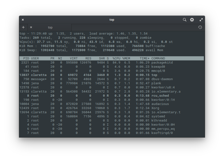
Top (above) is a popular interactive task manager for linux command line. Learn more with man top.

So going back to our example with fasta files and having quick look at them, you can send the results of head into interactive browser less:

head *fasta | less

Processing files

There are several tools in linux that allow you to process files in very efficient ways. Some more simple, some more complex (in fact up to the level of programming languages), but their basics are usually easy to master. The most useful tools range from sed or tr to awk and perl. Some of them are way too complex (e.g. perl) to cover here fully, so I will just introduce them at a level I consider useful.

sed

The sed command, i.e. the “stream editor” is used all the time in the work of bioinformatician. Stream is the stuff you send from stdout to stdin. The sed allows you to edit it, process it, format it, or almost whatever your imagination holds (if not, there is still awk and perl). You can think of it as find-and-replace feature from your Office suite, but on steroids. Most notably, sed can use regular expressions (regex) to filter and process your data.

Typical sed syntax could look like this:

sed 's/OLD/NEW/g' file.txt # substitute OLD with NEW in file.txt and print to stdout

This command takes a file.txt and substitutes (s) the pattern OLD with pattern NEW, globally (g), i.e. every occurrence on every line. If you omit the g, it will replace just the first occurrence of OLD on every line.

By the way, the slashes used for separating patterns are more of a convention - if you need something else, you can replace them. Consider this example, where you would replace slashes / with double-slashes //:

sed 's/\//\/\//g' file.txt # wait what?
sed 's#/#//#g' file.txt # aha ok!

In the first version we had to escape the slashes as special characters (by prepending them with backslashes \). By using a different separator we could avoid the issue entirely. A more realistic case would be for example to process filenames with paths in your script, that often contain slashes.

You can play around with sed by piping to it e.g. from the echo command:

echo Hello world! # prints Hello world!
echo Hello world! | sed 's/ /\t/' # replaces space with tabulator

Sed can also do much more than just simple find-and-replace operations - it can count lines based on a pattern, process every odd, even, or 71th line in your file and so on. It really gives you quite a power to select the right lines as well as processing capabilities. You can also chain several sed commands with pipes into a pipeline for even more complex processing.

tr

Tr is another tool for doing replacements of patterns in your files. I found it to be quite simple to use and more user friendly in some cases (for instance working with line breaks in sed can be little tricky, while tr is pretty straightforward).

The basic syntax of tr would look as follows:

tr "OLD" "NEW" file.txt # replace OLD with NEW in file.txt
tr -d "OLD" file.txt # delete OLD from file
tr " " "\t" file.txt # replace each space with a tabulator

Tr is not as popular in the online tutorials as sed is, probably because it’s little limited in what it can do when compared to sed. However it’s very simple to use and can be also chained by pipes into more complex processing tool, so feel free to play around with it.

AWK

AWK is not just a command, but a whole programming language. It’s designed to process text files, especially in tabular format, extract data and create reports.

Life in the commandline

There is no reason to go crazy from the command line. Quite a few programs were designed by pros and wizards to make your life in the command line much easier. From file managers and text editors to internet browsers and even music players.

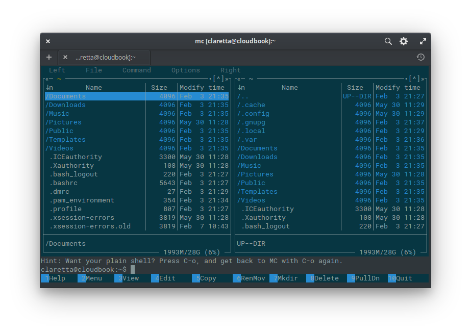
Midnight Commander - the savior

midnight commander

Start this advanced file manager with simple:

mc # launches Midnight Commander

After opening, you will see two panels listing content of current folder - you can use Tab to switch between the panels (mouse clicks also work here, which is kind of cool).

On the bottom you see 10 buttons with labels and numbers - the numbers correspond to keys on top row of your keyboard, labeled F1 - F10. So for example to copy file(s) between panels (if you open different folders in them) you just press F5. Easy :)

💡️ Tip: select multiple files with Shift (if you use ssh from Ubuntu) or Insert (Putty on Windows & Xubuntu terminal)

View (F3) and Edit (F4) are little miracles on their own - you can use View to see content of various files (as long as they are not binary, so it works on text files, fasta, fastq and even displays basic pdf and html files! - how cool is that? :))

Edit can open and modify many text files and scripts. In case of script files you get features like syntax highlighting etc.

💡️ Tip: sometimes (probably first time) after pressing F3 or F4 you are asked to select default viewer or editor. The natives of MC are easy to pick by name - mcview and mcedit. I’m talking about these in here.

Sometimes you need to run some regular commands when you have MC open. You can “minimize” MC with keyboard shortcut Ctrl+o (or C-o for short). You can later get back to MC with the same shortcut.

Text editors

MCedit

MCedit can even be started by itself, without the MC. For instance you can simply create new text file in the current directory by typing:

mcedit new.txt # opens empty new.txt file in the MC editor

You can edit existing files the same way, just type a name of some file in the folder to open it.

💡️ Tip: name completion with Tab key works as expected ;)

Nano

Very simple and popular command line text editor. The shortcuts at the bottom buttons work with Ctrl and the corresponding letter. So to e.g. exit nano editor you would press Ctrl+x (it will also ask you to save any changes). You can start it the same way as other editors:

nano new.txt # opens empty new.txt file in the nano editor

nano text editor

Other editors

There are other editors, popular with linux gurus and commandline wizards, such as Vi / Vim or Emacs. Although they are powerful, in my opinion they are too complicated for beginners’ use (I use mcedit most of the time, or in case I need something more sophisticated, I switch to graphical editor, such as Sublime text). But it’s good to know they exist. So if you see some online tutorial, which uses vim command to edit a text file, you can replace vim with some other editor you prefer. Vi/vim is very common in online tutorials as it’s an editor that is installed on every linux computer on the planet, which is not the case for other editors. However there is a way out - later I show you how to install nano if it’s missing on your system (most modern systems like Ubuntu have nano though).

Keep the work running

When you login to some linux server, you usually plan to run some kind of pipeline or analysis, that usually runs for several hours or days, so you don’t want to bother your own computer with it. However if you just login and enter your commands, you will soon find out that after you logout, your session was interrupted and all your programs were closed. Just like if you turned off your own computer, your programs would also close.

But do not despair - there are several ways to keep your jobs running in your absence and this section will be all about how to do it.

Disown & nohup

Probably the most simple way is to complement your command with either nohup or disown. These two tools do similar thing, but in a bit different way - in practice nohup has to be entered before your main command, while disown is used after your main command. In layman’s terms the command nohup prevents the system to send “quit” (hup) message to kill your program, while disown changes ownership of your program’s process so it doesn’t quit when you logout.

You would use them as follows:

command & disown # keeps command running after logout
nohup command & # another way to run command after logout

For example:

bwa mem ref.fa reads.fq > aln-se.sam & disown
nohup bwa mem ref.fa reads.fq > aln-se.sam &

💡️ Tip: the & symbol moves the command into background so you can input other commands (e.g. disown). It doesn’t let you logout from HPC without interrupting your job (on its own), but it allows for some rudimentary multitasking.

If you find that nohup doesn’t work with some programs, it might be because programmers of the software in question can change nohup behaviour. In such case disown should be a safer option.

Terminal multiplexers

Terminal multiplexers are incredible tools, that allow starting multiple programs, run them in parallel in separate “windows” or “workspaces”, switch between them, and they also keep your programs running when you detach from your session on logout. Actually you may even skip detaching and just close the window and they will keep running your programs - this might be especially helpful if you connect from a weak or patchy network (e.g. train), so that random disconnection doesn’t ruin your work. The two most popular examples are GNU-screen and tmux.

GNU-screen

GNU-screen is commonly installed on servers and HPCs, because it’s so helpful. You can start new screen sessions or list and reconnect to already active sessions with these commands:

screen -S transcriptome-pipeline # creates new (named) screen
screen -ls # lists available screens (with PIDs)
screen -d -r PID # detach and reattach to screen with PID

Typically you would connect to a HPC, reconnect to one of your screens or start a new one and start some long-running script. You can use keyboard shortcuts to switch between different windows and so on.

These shortcuts always start with a prefix key Ctrl+a combo (C-a for short) followed by some other key or combination of keys. For example to create new workspace you would press C-a, release both and then press c. Some shortcuts use capital letter after pressing C-a - that just means you hold Shift when you press the letter. For instance the shortcut to start logging your screen into a file is C-a H, or Ctrl+a followed by Shift+h, to be more explicit. If the second key contains Ctrl, then you don’t have to release it after C-a - e.g. switching between last two workspaces is done by holding Ctrl and tapping two times the letter a (C-a C-a).

Some of the shortcuts I find most usefull are these:

C-a c = create new workspace
C-a C-a = switch between last two workspaces (ala Alt+Tab)
C-a “ = show list of workspaces inside current screen session
C-a n/p = switch to next/previous workspace
C-a d = detach from a screen session
C-a ? = help

You can find more info in the man screen page (if you don’t have it on your local computer, you can still read it on the HPC/cluster where you connect to).

ℹ️ Note: I noticed that some programs (especially MC) may work slightly differently inside screen session than they would do normally. For example on some HPCs the mouse input is ignored and you have to use keyboard for scrolling (arrows, PgUp & PgDn) or opening menu (F9) in MC. Also you won’t see history of your commands when you minimize MC with Ctrl+o (but you can still browse previous commands with arrow up). Other programs, like emacs, may be also affected. However I’ve only seen this on a few HPCs.

Tmux

Tmux is very similar in functionality to screen and it’s good to know about it in case screen is not installed on your HPC system. The basic commands are similar to screen:

tmux new # starts new session with default name (0, 1, ...)
tmux new -sAnalysis # start new session named "Analysis"
tmux attach # attach to last session
tmux attach -tAnalysis # attach to session named "Analysis"

As allways - more info in man tmux, you can also find more in tmux online tutorial.

The prefix key combo for tmux is Ctrl+b. For example C-b d will detach the current session. You can check other shortcuts for tmux with C-b ?.

Tmux has one advantage over screen - it can be installed rather easily, in case both tools are missing on your HPC, thanks to conda manager that I discuss later.

Qsub / Bsub & co.

The options above serve well on machines that are used in university courses or managed by someone you know in person. However if you ever use big professional cluster like IT4Innovations, MetaCentrum or Elixir, you will find they use specialized software to manage their computing jobs (also because they have to manage vastly more users that compete for resources).

The two systems I’ve encountered are qsub (from PBS system) and bsub, both work in very similar way - you enter a qsub/bsub command followed with parameters for number of cores you want, memory you need, time you plan for the job etc. and then follows name of a script file with your actual job. These big profi clusters usually have proper documentation for preferred use of these commands in place, so I will leave it to them :)

Here are just a few quick example qsub commands to get you started:

qsub -N Job_name -l nodes=1:ppn=24:mem=32GB,walltime=48:00:00 job_script.sh # job submission with in-line PBS parameters (1 node, 24 cores, etc)
qstat -u username # check status of username's jobs
qstat # status of all jobs
qstat -a # status of all jobs with more info
qdel JOB.ID # kill job with JOB.ID

ℹ️ Note: There are several implementations of the PBS system, including popular open-source TORQUE or commercial PBS Pro (used e.g. by IT4Inovations). These implementations may differ in how they use parameters. Here I’m showing the parameters for TORQUE, with details available here.

Interactive session in PBS

What if you want to test commands to prepare your job script, but you don’t want to block the login node with your intensive processes? Easy, PBS supports interactive jobs. You can start it like this:

qsub -I -l nodes=1,walltime=3:00:00 # starts interactive session on 1 computation node, for 3 hours

After a moment PBS will start a session for you on a computation node, where you can test your commands without blocking the login node. It’s good idea to set a walltime limit so the job is ended when you no longer need it. You can also end the job by typing exit, pressing Ctrl+d or terminate it with qdel command as above.

You can also check the manual pages:

man pbs # manual page of PBS system
man qsub # manual page for qsub command

Installing software

There are many ways to install software on linux system, however the most important question for you is whether you have admin (root) privileges or not (I assume you have internet connection, otherwise you have bigger problem at hand). If you use linux on your own desktop/laptop, you almost surely have these privileges. That means you can easily install software from online repositories with package managers like apt, yum, or pacman. However in case of linux servers or HPCs (High Performance Computers) needed for many resource-intensive analyses and pipelines, the chances are you don’t have admin rights.

Big computing centres like IT4Innovations, Elixir or MetaCentrum have their own way of handling your software needs. They usually have software modules available, which you can load to your environment and then use packages from these modules. Again, I will leave it to proper documentation of these computing centres to tell you how to use these modules.

There are however still cases where you need to install software on your own:

On smaller HPCs, run by e.g. university, usually managed by one or few person(s).
On big clusters, if the software in their modules is old / outdated (or you just need different version).

Historically, in such cases your options would include (based on my experience, in order of preference):

Email the admin and ask him to install the package you need. Do a bit of googling on what version you need and if it depends on other packages (“dependencies”).
Some packages run without installation, then you are in luck. For example all java programs run without installation and Java environment is usually pre-installed on HPCs and clusters. Downside is - they are Java programs.
You could compile the package from source into your ho me directory (non-system-wide installation). This process may vary wildly in terms of time, trouble and/or pain. Some packages are designed to compile with one command, others will make you hunt for dependencies all over the internet. Some just fail entirely for reasons beyond your reach. Then, your only hope is the admin from 1.

But there are new better options, coming from this century :)

Scientific package managers

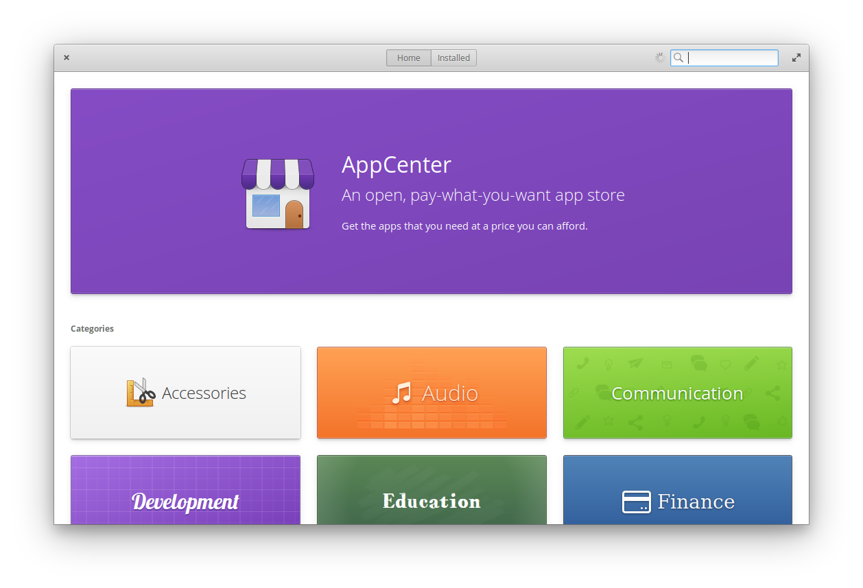
Package managers are very common on Linux distributions - they make installing software easy by connecting to curated repositories, from which you can download and install any available software using these managers. Some managers aim at general users and look like Google Play store (see e.g. elementary AppCenter below), other managers are focused on power users.

elementary AppCenter

Most of the general package managers present in Linux distributions require root (admin) privileges. However several package managers have been developed specifically for scientists and for use on HPCs and clusters without such privileges. These include conda and linuxbrew. Most programs are available via both managers, however I found few edge cases when a package was only found in one of them. ~~However it’s possible to install and use both at the same time.~~ Update: I haven’t tested this rigorously, but I would be careful using both on the same machine because of the PATH variable (which also depends on if you include any of them in the system path). I used both on the same machine to some extent by including only one (conda) in the system PATH.

Even though these managers aim at HPCs, you can also use them on your own laptop. And it’s often a good idea to do so - you will have the same versions of packages on both laptop and HPC, so you don’t have to worry about incompatibility of your scripts with different versions of packages. It’s then very easy to develop and test your scripts and pipelines, before running them on HPC and full data for weeks.

Conda

conda software manager

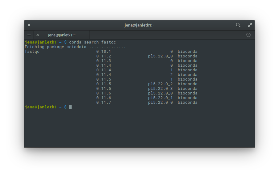
Conda started as a package manager to distribute python packages for data science, as part of Anaconda project. However since then it grew into general purpose package manager with several software repositories (channels) for science and bioinformatics, the most important being Bioconda. These days, conda will let you install a lot of scientific software, including:

Python 2 & 3, Biopython, pip, spyder, jupyter, …
R, Bioconductor, RStudio, …
Perl & Bioperl, …
C, C++, gcc compiler, …
Java (OpenJDK, …)
Bioinformatic packages such as
- QC software (fastqc, multiqc, afterqc)
- Trimmers (trimmomatic, …)
- Assemblers (abyss, soapdenovo2, spades, …)
- Mappers (bwa, bowtie2, …)
- Variant callers (samtools, GATK, freebayes, …)
- NGS viewers (IGV)

You can get conda in two different ways: either you download and install the full Anaconda distribution (recommended if your workflow is python-heavy) or you download Miniconda, which includes only the conda package manager and few supporting packages (recommended if you don’t care about python, e.g. if you use R or other software). Either way you get it, you can then use the conda manager to install whatever other software you want (including full Anaconda, if you started with miniconda), add new repos (channels) and get quickly back to your work.

Conda even allows you to install nano editor. It’s as simple as:

conda install nano # installs nano from main repository
conda install -c conda-forge nano # installs newer version of nano editor from the conda-forge channel

Conda-forge is probably the most important channel for all things conda. You will find a lot of useful packages there, lot of which are missing from default channels or only present in older version (as does nano in the example above). The Bioconda channel depends on conda-forge to build a lot of the packages. This means that if you install packages from bioconda channel, you should also include conda-forge. The easiest way is to just add both channels to conda configuration using conda config --add channels command, which you can find in the bioconda instructions. After adding the channels, you don’t have to specify them anymore with the -c option.

Another useful package in conda-forge channel is tmux, discussed before. You can install it with this command:

conda install -c conda-forge tmux

Linuxbrew

Linuxbrew is a port of popular Homebrew package manager from macOS. It is based on ruby instead of python, however as with conda, the language used is not important to the end user. It also lets you install software on HPCs and clusters without root (admin) privileges, using its own repositories, called taps, to download and install software. The most useful tap for bioinformatics is BrewSci-bio.

Sequences everywhere

Most sequencing projects start with raw data from sequencing centre, typically in FastQ format. The common file extensions are fastq or fq, or in case of files compressed by gzip, the extension would be e.g. fq.gz. Some sequencing centres send the data with txt.gz extension, but the format is still gzipped fastq.

Data overview

The FastQ format consists of four lines per each read, meaning we can count lines and divide by 4 to figure out number of reads sequenced. With uncompressed fastq, this could be as simple as:

wc -l file.fq # counts number of lines in file.fq

For instance paired-end (PE) data usually come in two files and they should have the same number of lines. We can use wildcards to check both files with one command:

wc -l sequences*.fq # counts number of lines in files such as sequences_F.fq & sequences_R.fq

With compressed files, as is usually the case due to their size, it gets little more tricky. The wc tool doesn’t work with compressed files, so we have to use zcat (cat for gzipped files) or other method to uncompress the data first. The command zcat also has to uncompress the whole file before wc can count lines, so it can take considerably longer. The simplest command would look like this:

zcat file.fq.gz | wc -l # uncompress file.fq.gz on the fly and count lines

However with PE data it’s not as simple, as zcat would concatenate them (just like cat would) and wc -l would give us just number of lines in the concatenated file, so we should use for loop instead of just wildcards:

for f in file*.fq.gz
do
    zcat $f | wc -l
done

Or on one line:

for f in file*.fq.gz; do zcat $f | wc -l; done

So now you know two ways to write for loop in bash - didn’t even hurt, did it ;)

But in case you are wondering: we used wildcard file*.fq.gz to select our files, then the for loop assigns them one by one to the variable f. We then call this variable by using it with the dollar sign, like $f. Then the for loop uses keywords like do and done at the beginning and the end of our loop, respectively. And in the one-liner version, you have to put a few semicolons ; to delimit lines or blocks of code. That’s pretty much it :)

There are actually simpler ways to do this even with wildcards. For example you could use zgrep -c to count lines with some pattern present on all lines, such as beginning of line ^ or empty string ''.

zgrep -c ^ file*fq.gz # counts all lines in each file matching the wildcard
zgrep -c '' file*fq.gz # again counts all lines in each file

However, you will still need for loops to process your files with specialized bioinformatics softwares. For instance most trimmers or mappers (aligners) allow at most two files for primary input and wouldn’t work if you try to provide all your files in one step. You will need the for loop in the future.

💡️ Tip: you might be wondering now how many other tools you already know work with gzipped files just by appending z at the beginning of their name - the truth is, I only know about these two, zcat and zgrep. There might be more, but it’s not common to see them in the wild (i.e. on the internet).

Quality control (QC)

Playing with files like this is all fun and games, but if you want some real work done, you need something better. You want to understand the sequences, and the first thing is to check quality of the sequencing itself - i.e. if our sequences are real biology or full of technical artifacts.

FastQC

Probably the most widely used program for QC is FastQC. It has graphical window, or can be used from commandline if you have many files.

fastqc # start the program in graphical mode
fastqc *fq.gz # run the program on all fastq files in current folder

The first command opens a graphical window, where you select a file for QC using the menu. The second command runs the analysis on specified file, in this case all files in a directory that end with fq.gz. It will output the reports in html format, that you can open in any web browser.

💡️ Tip: to open graphical programs in ssh session (e.g. when connected to HPC), you have to add a parameter to the ssh command. The options are -X (no encryption), -Y (yes encryption) or simply -XY (encryption, unless it’s not supported). So you would connect e.g. using ssh -XY studentuser@genome.osu.cz.

MultiQC

MultiQC is a package designed to assess multiple samples at once. It uses output of FastQC and compiles an interactive report for all samples.

It is especially useful in projects that use reduced representation of genomes to scan large populations or hybrid zones, such as sequence capture (also known as targeted enrichment), RADseq (restriction-site associated DNA), GBS or similar methods.

AfterQC

AfterQC is a tool that can compile a QC report of your data, but also perform trimming of your reads based on various criteria.

However I’m personally careful to use this tool, as a lot of the trimming options are enabled by default and it’s quite tedious to switch off the ones you don’t want. There is an option to produce just the report without any trimming though.

Trimming

Speaking of trimming, it is usually the next step after QC. It is done to remove low-quality bases (or reads), artificial DNA (such as leftover sequencing adapters or PhiX spike-in), or just to trim reads to the same length (which might be required in some subsequent tasks, such as de novo assembly).

There are several popular trimming tools that typically use one of the two main approaches to trimming. Tools like Trimmomatic or fqtrim use sliding-window method to scan reads, while e.g. BBDuk uses k-mers to scan reads.

The importance of read trimming depends on what do you plan next with those reads. If you want to use those reads for de novo assembly, you have to perform trimming very carefully. If you just want to align (map) reads to assembled reference genome or transcriptome, then you can afford some suboptimal trimming, as mapping to reference will take care of some of your problems (e.g. adapters will not map to a reference that doesn’t contain their sequence).

De novo assembly

De novo sequence assembly is quite advanced topic so I will touch only briefly on a few aspects. Use the lectures of dr. Flegontov or other resources to get more in-depth knowledge of the topic.

The aim of assembly is to reconstruct long sequence of DNA from very short fragments, produced e.g. by Next-gen sequencing. For instance Illumina reads span from 75bp up to 300bp (as of 2018-19). Paired-end reads give extra power, but they are not nearly long enough - they allow reading of fragments from both ends, but Illumina still requires fragments around 700bp. So a specialized algorithms had been developed to use overlaps between many reads to create so called contigs - a somewhat longer pieces of DNA sequence, sometimes spanning whole genes.

The final goal of assembly is to produce a reference sequence, such as a genome, a transcriptome, or other, that can be then used for mapping (alignment).

Several quality packages exist to perform de novo assembly of your sequences, some more general, others more optimized to data of certain size (e.g. bacterial genomes) or type (e.g. RADseq).

Popular assemblers include Velvet, Abyss, SPAdes, SOAPdenovo2, or tadpole (from BBtools). These typically work with shotgun sequencing data, such as produced by whole-genome sequencing (WGS), RNAseq, or sequence capture. Rainbow is a popular assembler for RADseq data produced by the original protocol of Baird et al (2008).

Redundancy reduction

After assembly it’s often necessary to clean the reference from repetitive sequences, pseudogenes, paralogues, and other redundant sequences. One reason is to improve subsequent mapping, where multiple mapping candidates in the reference would dilute the coverage of our data. You also want to remove false signal from e.g. pseudogenes before you analyze data.

There are several approaches to deal with redundancy. Some popular packages include CD-Hit software or the MCL algorithm.

Quality assessment

After successful assembly and cleaning of the reference, one might want to see how the reference improved and if it can be improved further.

Scaffolding

Scaffolding typically follows the assembly step. The aim is to connect separate contigs into longer sequences, using e.g. paired-end (PE) data or some other source, e.g. mate pairs (MP). The contigs are connected by gaps, no new sequence data are added. This information on physical proximity of contigs is extracted from known length of fragments, that were sequenced from both ends (e.g. using PE or MP).

Scaffolding is useful for better understanding of expression, linkage (and LD in populations), and other useful features of sequencing data.

Mapping

More stuff soon, now I’m a bit busy :)