Getting taxonomy from NCBI with `R` & `rentrez`
Recently, I happened to work with Blast a lot. At some point we wanted to get some high-level taxonomy for our dataset. I’ve never done this, but I know the NCBI provides a query interface called Entrez, which can be accessed from command-line tools as well as from several programming languages. In R, you can query the Entrez system with the rentrez package. Here I describe the basics of getting taxonomy information with this package.
Let’s load our packages - rentrez and also magrittr (to get pipes for easier coding):
options(repr.plot.width=7, repr.plot.height=7, jupyter.plot_scale = 1)

library(magrittr)
library(rentrez)
Here is the list of available databases:
entrez_dbs() %>% print
 [1] "pubmed"          "protein"         "nuccore"         "ipg"
 [5] "nucleotide"      "structure"       "genome"          "annotinfo"
 [9] "assembly"        "bioproject"      "biosample"       "blastdbinfo"
[13] "books"           "cdd"             "clinvar"         "gap"
[17] "gapplus"         "grasp"           "dbvar"           "gene"
[21] "gds"             "geoprofiles"     "homologene"      "medgen"
[25] "mesh"            "nlmcatalog"      "omim"            "orgtrack"
[29] "pmc"             "popset"          "proteinclusters" "pcassay"
[33] "protfam"         "pccompound"      "pcsubstance"     "seqannot"
[37] "snp"             "sra"             "taxonomy"        "biocollections"
[41] "gtr"
The basic command to get taxonomy for an ID:
taxo <- entrez_summary(db="taxonomy", id="1219383")
str(taxo)
List of 13
 $ uid             : chr "1219383"
 $ status          : chr "active"
 $ rank            : chr "species"
 $ division        : chr "g-proteobacteria"
 $ scientificname  : chr "Acinetobacter boissieri"
 $ commonname      : chr ""
 $ taxid           : int 1219383
 $ akataxid        : chr ""
 $ genus           : chr "Acinetobacter"
 $ species         : chr "boissieri"
 $ subsp           : chr ""
 $ modificationdate: chr "2015/07/31 00:00"
 $ genbankdivision : chr "Bacteria"
 - attr(*, "class")= chr [1:2] "esummary" "list"
You can extract just the part you want with $:
entrez_summary(db="taxonomy", id="1219383")$division
‘g-proteobacteria’
Search & links
But suppose for a moment that we do not have the staxids - can we still get this information with e.g. accession number (saccver or similar)?
Of course we can!
Let’s say we want to search the taxonomy for accession number WP_092748568.1. We start by searching the protein database, where the accession number comes from:
entrez_search(db="protein", term="WP_092748568.1")
Entrez search result with 1 hits (object contains 1 IDs and no web_history object)
 Search term (as translated):
We see there is 1 hit, but it doesn’t show any information about it - yet. You could save the result of the query into an object and expect it with str() - or we can use magrittr pipe directly on the query:
entrez_search(db="protein", term="WP_092748568.1") %>% str
List of 5
 $ ids             : chr "1224730548"
 $ count           : int 1
 $ retmax          : int 1
 $ QueryTranslation: chr ""
 $ file            :Classes 'XMLInternalDocument', 'XMLAbstractDocument' <externalptr>
 - attr(*, "class")= chr [1:2] "esearch" "list"
Now we can see the internal NCBI ID of this item, under the $ids slot. We can now look up what other information is linked to this ID:
ncbi_id <- entrez_search(db="protein", term="WP_092748568.1")$ids

entrez_link(dbfrom="protein", id=ncbi_id, db="all") %>% str
List of 2
 $ links:List of 16
  ..$ protein_cdd                    : chr [1:16] "415644" "399551" "395146" "236886" ...
  ..$ protein_cdd_concise_2          : chr "163712"
  ..$ protein_cdd_specific_2         : chr "163712"
  ..$ protein_cdd_summary_nonpublic  : chr [1:13] "395146" "223824" "215328" "215003" ...
  ..$ protein_cdd_superfamily_2      : chr "415644"
  ..$ protein_nuccore                : chr "1224732327"
  ..$ protein_protein_cdart_summary  : chr "1224730548"
  ..$ protein_sparcle                : chr "10169238"
  ..$ protein_taxonomy               : chr "1219383"
  ..$ protein_bioproject             : chr "224116"
  ..$ protein_cdd_summary            : chr [1:16] "415644" "399551" "395146" "236886" ...
  ..$ protein_nuccore_wp             : chr "1224732327"
  ..$ protein_protein_cdart          : chr "1224730548"
  ..$ protein_protein_cdart_summary_2: chr "1224730548"
  ..$ protein_protfam                : chr [1:7] "326225" "315947" "246230" "246128" ...
  ..$ protein_taxonomy_wp2species    : chr "1219383"
  ..- attr(*, "class")= chr [1:2] "elink_classic" "list"
 $ file :Classes 'XMLInternalElementNode', 'XMLInternalNode', 'XMLAbstractNode' <externalptr>
 - attr(*, "content")= chr " $links: IDs for linked records from NCBI\n "
 - attr(*, "class")= chr [1:2] "elink" "list"
As we can see, there is a link to the taxonomy database, showing us an id “1219382”. Now we can reuse this ID in our query:
our_id <- entrez_link(dbfrom="protein", id=ncbi_id, db="all")$links$protein_taxonomy

entrez_summary(db="taxonomy", id=our_id) %>% str
List of 13
 $ uid             : chr "1219383"
 $ status          : chr "active"
 $ rank            : chr "species"
 $ division        : chr "g-proteobacteria"
 $ scientificname  : chr "Acinetobacter boissieri"
 $ commonname      : chr ""
 $ taxid           : int 1219383
 $ akataxid        : chr ""
 $ genus           : chr "Acinetobacter"
 $ species         : chr "boissieri"
 $ subsp           : chr ""
 $ modificationdate: chr "2015/07/31 00:00"
 $ genbankdivision : chr "Bacteria"
 - attr(*, "class")= chr [1:2] "esummary" "list"
Cool. Now we can get taxonomic information for one sample. But what if we have 5 - or 5000?
Yes we can! In particular, we can supply most of the functions we used with a vector of IDs instead of just one ID. But let’s get some data first.
Real data - Blast output
I started with a blastp output in tabular format with few extra columns - in particular the accession number and Tax ID, so you need at least this: -outfmt '7 saccver staxids' to get taxonomy IDs for your blast hits (note that saccver is part of standard blast output, which can be specified with the std format keyword).
Note: You can also ask blast to provide e.g. scientific names, however so many of them were missing in my queries that I just gave up on using that.
Since staxids can include multiple IDs separated by ;, I had to process the data slightly with awk before they were ready:
# take columns 2 (saccver) and 13 (staxids) from blast output table (skipping header)
awk -F"\t" '!/#/ {print $2, $13}' blastp_outfmt7_std_staxids.tsv > blastp_saccver_staxids.txt

# expand items with multiple staxids row-wise by replacing ";" with "newline+saccver+space"
awk '{gsub(/;/, "\n"$1" ", $2); print $0}' blastp_saccver_staxids.txt > blastp_saccver_staxids_expanded.txt
Now we are ready to load the data into R:
taxa <- read.table("blastp_saccver_staxids_expanded.txt", h=F, sep=" ") #, stringsAsFactors = T)
colnames(taxa) <- c("acc", "id")
str(taxa)
'data.frame':	13842 obs. of  2 variables:
 $ acc: chr  "WP_092748568.1" "WP_023273437.1" "WP_023273437.1" "WP_088823490.1" ...
 $ id : int  1219383 1219382 1392540 1229165 29545 2691581 1907941 86304 203122 2675457 ...
Test data (10 ids)
So far we used the function str() to see results of our queries and to figure out which data to extract with $. Of course this is not practical for bulk queries with multiple IDs. For this reason there is a helper function - extract_from_esummary(). It accepts a list of results from your query and a name of the field you want to extract. We can pipe into it as usual:
entrez_summary(db="taxonomy", id=taxa$id[1:10]) %>% extract_from_esummary("division") %>% print
           1219383            1219382            1392540            1229165
"g-proteobacteria" "g-proteobacteria" "g-proteobacteria" "g-proteobacteria"
             29545            2691581            1907941              86304
"b-proteobacteria" "b-proteobacteria" "g-proteobacteria" "g-proteobacteria"
            203122            2675457
"g-proteobacteria" "b-proteobacteria"
Full data (~90k ids)
The basic command to extract taxonomy through Entrez looks like this:
entrez_summary(db="taxonomy", id=taxa$id) %>% extract_from_esummary("division")
I cannot actually ask Entrez to give me all data at once - they limit queries to certain (unknown) size. After a bit of experimenting, I found I can get 400 items at a time. So in reality, we need to divide the data into chunks and loop over the chunks to get the full dataset.
Note: the
rentreztutorial says I should use web history feature for large queries, however this option has the same limit on items as getting them directly. So I skipped web history and just got the stuff I needed directly.¯\_(ツ)_/¯
nrow(taxa)
(nrow(taxa)/400) %>% round
13842
35
Divide data into chunks of 400 IDs and store them in a list:
id_list <- (seq_along(taxa$id)/400) %>% ceiling %>% split(taxa$id,.)
Use lapply to loop over the list using our extraction command:
all_division <- lapply(id_list, function(x) {entrez_summary(db="taxonomy", id=x) %>%
                             extract_from_esummary(., "division")})
Warning message:
“ID 332056 produced error 'cannot get document summary'”
Warning message:
“ID 2044510 produced error 'cannot get document summary'”
Warning message:
“ID 2694937 produced error 'cannot get document summary'”
Warning message:
“ID 2024862 produced error 'cannot get document summary'”
Warning message:
“ID 2660640 produced error 'cannot get document summary'”
Warning message:
“ID 2660639 produced error 'cannot get document summary'”
Warning message:
“ID 2731243 produced error 'cannot get document summary'”
Warning message:
“ID 1330039 produced error 'cannot get document summary'”
Warning message:
“ID 262776 produced error 'cannot get document summary'”
Warning message:
“ID 2529841 produced error 'cannot get document summary'”
Warning message:
“ID 2731248 produced error 'cannot get document summary'”
Warning message:
“ID 2731248 produced error 'cannot get document summary'”
Warning message:
“ID 2529844 produced error 'cannot get document summary'”
Warning message:
“ID 332056 produced error 'cannot get document summary'”
Warning message:
“ID 2529844 produced error 'cannot get document summary'”
Warning message:
“ID 2027912 produced error 'cannot get document summary'”
Warning message:
“ID 2660639 produced error 'cannot get document summary'”
Warning message:
“ID 2660640 produced error 'cannot get document summary'”
Warning message:
“ID 262776 produced error 'cannot get document summary'”
Warning message:
“ID 262776 produced error 'cannot get document summary'”
Now we can see the taxonomic representation in our dataset.
Note the
magrittr“T-pipe”%T>%in the following command - it alows side-piping data into a plot, but also reusing it (here for printing the output oftable). The extra pipes are the main reason I use the originalmagrittrpackage instead of e.g.dplyr.
all_division %>% unlist %>% table %T>% pie %>% sort(decreasing=T)
.
     g-proteobacteria      e-proteobacteria      b-proteobacteria
                 4419                  2066                  1749
           firmicutes      a-proteobacteria    CFB group bacteria
                 1671                  1418                   867
             bacteria         high GC Gram+        enterobacteria
                  483                   302                   193
     d-proteobacteria         cyanobacteria
                  176                   140                    65
       proteobacteria          GNS bacteria        euryarchaeotes
                   52                    51                    44
      verrucomicrobia               archaea        planctomycetes
                   43                    20                    18
          spirochetes        actinobacteria        kinetoplastids
                   18                     7                     6
green sulfur bacteria        crenarchaeotes         thermotogales
                    5                     3                     2
          ascomycetes               beetles            chlamydias
                    1                     1                     1
    choanoflagellates
                    1
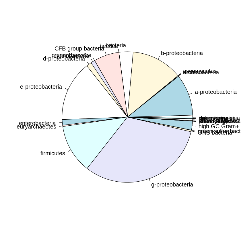
Wow, pretty… ugly. Let’s see what ggplot2 can do..
ggplot, just for fun
library(ggplot2)
df <- all_division %>% unlist %>% table %>% as.data.frame

colnames(df) <- c("Taxon", "Freq")
head(df)
| Taxon | Freq | |
|---|---|---|
| <fct> | <int> | |
| 1 | 65 | |
| 2 | a-proteobacteria | 1418 |
| 3 | actinobacteria | 7 |
| 4 | archaea | 20 |
| 5 | ascomycetes | 1 |
| 6 | b-proteobacteria | 1749 |
ggplot(df, aes(x = "", y = Freq, fill = Taxon)) +
  geom_col() +
  coord_polar(theta = "y")
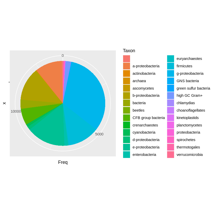
It is much nicer looking, but I actually have a problem distinguishing the different colours in the plot. I am colourblind, sure, but I think there is just too many colours for anyone to handle.
df$Taxon %>% unique %>% length
28
28 categories - that’s a lot! Well I think for this amount of data the base R is better - by default. There might be a way to improve both plots, but this is not the time nor place. See you next time 😉️